This post covers some of the basic R data frame analysis functions. I’ll demonstrate how some of these functions work with matrices too.
I’ve used the CheckWeight data set which comes out-of-the-box with the R programming runtime.
data(“ChickWeight”)
Type the Data Frame Name
The most basic method for evaluating the CheckWeight data frame is to simply type the data frame name after loading it:
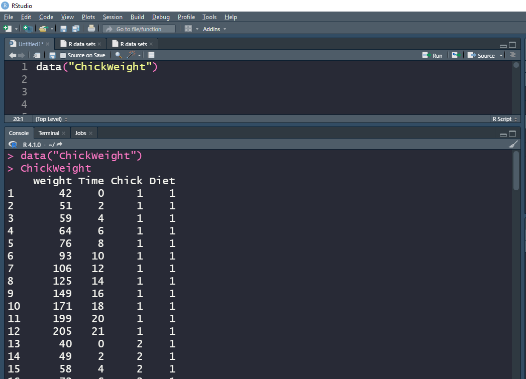
Here, we see the index and then column names. Note that a detailed explanation of the ChickWeight data frame can be found on the R documentation site. Briefly though, we’re looking at a unique identifier for every chicken (Chick) on a given diet (Diet). The metrics are then, the chicken’s weight over a given number of days (Time) for that specific diet. The chickens happen to be ordered by their final weight on the diet.
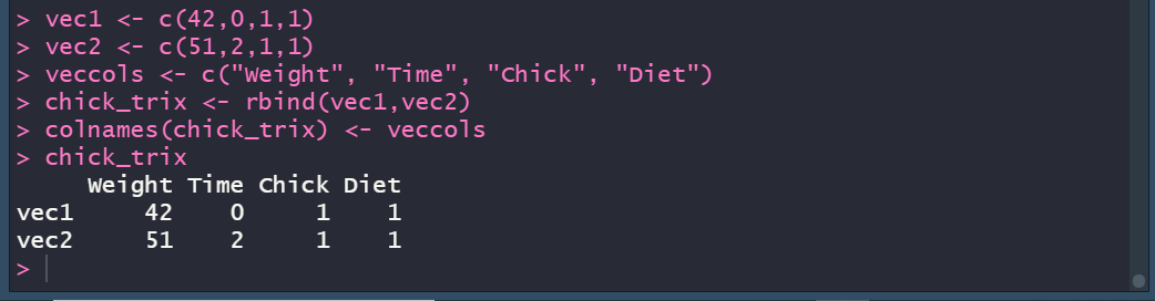
Typing the object name also works as the basic method for analyzing a matrix too of course:
A Look at the Data Frame Type
A data frame is both of type list and data.frame.
> typeof(ChickWeight) # I was not expecting “list” to be the output of this call
[1] “list”
> is.list(ChickWeight)
[1] TRUE
> is.data.frame(ChickWeight)
[1] TRUE
> is.list(chick_trix)
[1] FALSE
> is.matrix(chick_trix) # a matrix is only a matrix; not a list and a matrix
[1] TRUE
Counting Rows and Columns
To count rows and columns, the R language provides nrow and ncol respectively. These functions work the same for data frames and matrices:
> nrow(ChickWeight)
[1] 578
> nrow(chick_trix)
[1] 2
> ncol(ChickWeight)
[1] 4
> ncol(chick_trix)
[1] 4
First and Last Records with Head and Tail
Two simple methods available for R data frame analysis are the head and tail function, and these also work on the matrices.
> head(ChickWeight)
weight Time Chick Diet
1 42 0 1 1
2 51 2 1 1
3 59 4 1 1
4 64 6 1 1
5 76 8 1 1
6 93 10 1 1
> head(chick_trix)
Weight Time Chick Diet
vec1 42 0 1 1
vec2 51 2 1 1
> tail(ChickWeight)
weight Time Chick Diet
573 155 12 50 1
574 175 14 50 1
575 205 16 50 1
576 234 18 50 1
577 264 20 50 1
578 264 21 50 1
> tail(chick_trix)
Weight Time Chick Diet
vec1 42 0 1 1
vec2 51 2 1 1
> head(ChickWeight,n=10)
weight Time Chick Diet
1 42 0 1 1
2 51 2 1 1
3 59 4 1 1
4 64 6 1 1
5 76 8 1 1
6 93 10 1 1
7 106 12 1 1
8 125 14 1 1
9 149 16 1 1
10 171 18 1 1
> head(chick_trix, n=10)
Weight Time Chick Diet
vec1 42 0 1 1
vec2 51 2 1 1
The last test was to check what happens if the number “n” exceeds the count of available records. As seen, the head and tails function will execute gracefully and simply show what’s available.
Viewing Detailed Structure Information
The str (i.e. structure) function is a bit more complex than the previously covered functions.
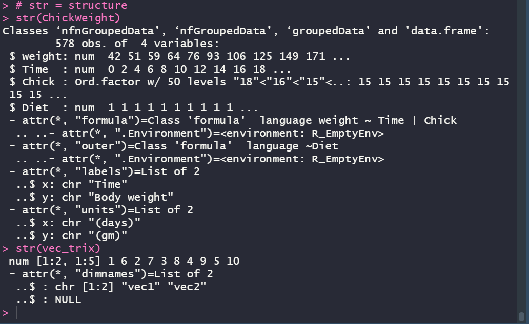
Some of the data is pretty straightforward. The weight column is a number column, and the output shows some representative values. Same with the Time column; it is a number value and the output is showing some relative values.
The “Ord.factor” output for the “Chick” column is much more interesting. Basically, R has figured out that the value is representing a grouping of information, and it has assigned a grouping number that can be referenced. It is an “ordered factor” as explained in the opening of this post that the chickens are grouped and ordered within each diet sample. What makes this example a bit obtuse is that the “Chick” column value is numerical. Take a look at the R data set, “InsectSprays”
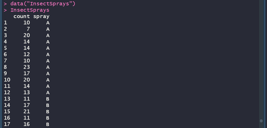
You can see the spray values are “A”, “B”, “C”, and beyond. So, when running str on this data frame, it is much more apparent what R is doing for us:
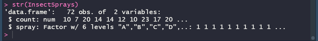
Now the concept of factor becomes more obvious. The data set has 6 unique “spray” values: A, B, C, D, E, and F. R has represented each of these groupings with a number (i.e. 1, 2, 3, 4, 5, and 6) which will be useful for selecting and filtering data.
R Data Frame Analysis with Summary
Last, but not least, let’s look at the summary function:

Here we see some interesting metrics: maximum values for given columns like weight and count alongside median and quarterly / percentile breakdowns. But, in closing, there is one more piece of data that really drives home that concept behind the Factor values covered above. Though not listed by their numerical representation, we can see clearly how R was able to figure out they were groupings and provided us with a count: there were 12 sample entries for spray A and all of the other sprays. Understanding that information is key to ensuring that a given sample wasn’t over-or-under represented.
More to come soon…
Categories: R Programming
Leave a Reply