This post covers matrix fundamentals in R programming. Working with matrices in R is a huge topic with complete documentation found at https://cran.r-project.org/doc/manuals/r-release/R-intro.html#Arrays-and-matrices.
My post will cover just the basics:
- Creating matrices
- Indexing and accessing matrices
- Options for working with column and row names
Creating Matrices
There are a few ways to create a matrix in R. Most commonly used, from what I’ve read, are rbind() and cbind(), but there’s also the less used matrix() which I’ll cover first.
Using the matrix() Function
Consider the following code:
by.matrix <- matrix(1:10,nrow=2,ncol=5)
by.matrix
This creates a ten-element matrix that is created by wrapping the series (1:10). The series is distributed vertically, moving across column-by-column:
> by.matrix <- matrix(1:10,nrow=2,ncol=5)
> by.matrix
[,1] [,2] [,3] [,4] [,5]
[1,] 1 3 5 7 9
[2,] 2 4 6 8 10
The distribution can be reversed, and flow row-by-row, by specifying byrow=T
> rowsby.matrix <- matrix(1:10, nrow=2, ncol=5, byrow=T)
> rowsby.matrix
[,1] [,2] [,3] [,4] [,5]
[1,] 1 2 3 4 5
[2,] 6 7 8 9 10
Using the rbind() Function
Using rbind() to create matrices in R is more intuitive because data often comes in a tabular format. That’s as opposed to wrapping a linear vector as seen above. For my testing, I used data from https://www.epa.gov/climate-indicators/climate-change-indicators-sea-level

The data above would reasonably be converted into a matrix where every row of data represents the CSIRO – Adjusted sea level (inches), CSIRO – Lower error bound (inches), CSIRO – Upper error bound (inches), and NOAA – Adjusted sea level (inches) for every year.
In advance, I set myself up with a vector containing the years and value-labels for each entry. I’ll show how that’s used later in this blog post. Here are manual entries for a subset of the data:
> years.recorded <- c(2006, 2007, 2008, 2009, 2010)
> value.labels <- c(“CSIRO – Adjusted sea level (inches)”, “CSIRO – Lower error bound (inches)”, “CSIRO – Upper error bound (inches)”, “NOAA – Adjusted sea level (inches)”
years.recorded
[1] 2006 2007 2008 2009 2010
value.labels
[1] “CSIRO – Adjusted sea level (inches)” “CSIRO – Lower error bound (inches)”
[3] “CSIRO – Upper error bound (inches)” “NOAA – Adjusted sea level (inches)”
Now, I can take those data and create a matrix using rbind()
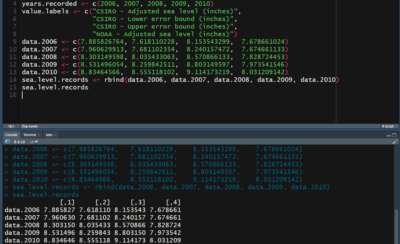
I don’t like these labels. The “data.*” style wouldn’t look good in a plot, and the anonymous labels on the columns have no meaning as they’re just integers. As noted above, I’ll be demonstrating how to change labels later in the post.
Using the cbind() Function
Above, we see rbind() in action. Briefly, the only difference between rbind() and cbind() is that the latter organizes data in a columnar fashion:
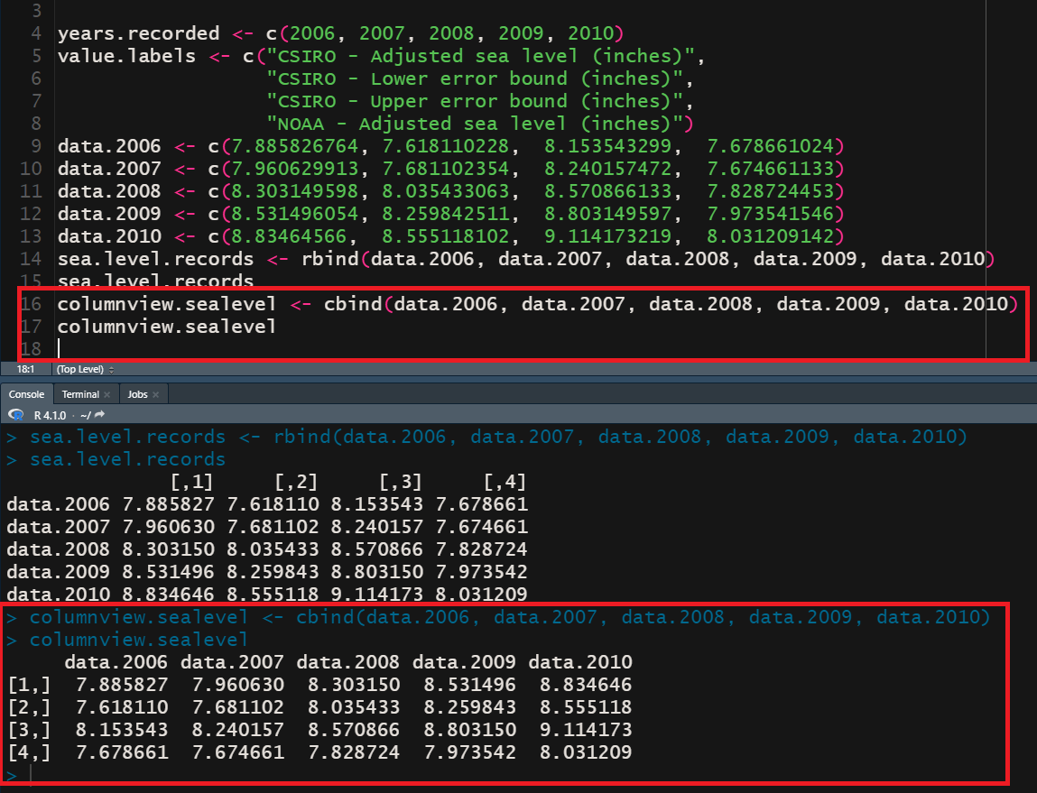
Previously, the year was represented on the row axis (i.e. axis 0), and now it has been transposed to the column (i.e. axis 1).
Indexing and Accessing Matrix Data
Moving forward with the first matrix, sea.level.records…let’s see how to index and access data. I’m going to improve this in the next section but first want to cover the default behavior.
Earlier, I created matrices using rbind() and cbind(). By default, the rows or columns (respectively) picked up the name of the vector while the opposite access remained “anonymous”. In the current state, that gives me basically two syntax options for accessing the elements of the matrix: by using the default-assigned names or by always using integer index values.
With the former, I mean that I can do the following:
> sea.level.records[“data.2006”,]
[1] 7.885827 7.618110 8.153543 7.678661
> sea.level.records[“data.2007”,]
[1] 7.960630 7.681102 8.240157 7.674661
> sea.level.records[“data.2008”, 2]
data.2008
8.035433
The synonymous syntax using the latter, integer only indexes, is as follows:
> sea.level.records[1,]
[1] 7.885827 7.618110 8.153543 7.678661
> sea.level.records[2,]
[1] 7.960630 7.681102 8.240157 7.674661
> sea.level.records[3, 2]
data.2008
8.035433
Also, I can exclude the row and just specify the column and the results are as expected. However, there is an option to apply row and column names so that we can reference the data similar to a dictionary as seen below.
Setting Matrix Column and Row Labels
The first thing to note is that I can do what I’m about to demonstrate to vectors and matrices. That is, to specifically set element names:
> temp.2006 <- rep(data.2006)
> names(temp.2006)
NULL
> names(temp.2006) <- c(“CSIRO – ASL”, “CSIRO – LEB”, “CSIRO – UEB”, “NOAA – ASL”)
> temp.2006
CSIRO – ASL CSIRO – LEB CSIRO – UEB NOAA – ASL
7.885827 7.618110 8.153543 7.678661
> temp.2006[“CSIRO – ASL”]
CSIRO – ASL
7.885827
Above, I replicated the data.2006 vector and then demonstrated how the names property on that new vector was NULL. Afterwards, the element names can actually be set using that same names() function.
Not surprisingly, there are analogous functions for matrices: colnames() and rownames(). So, to set up the matrix similarly, I executed the following:
> colnames(sea.level.records) <- c(“CSIRO – ASL”, “CSIRO – LEB”, “CSIRO – UEB”, “NOAA – ASL”)
> rownames(sea.level.records) <- c(2006, 2007, 2008, 2009, 2010)
> sea.level.records
CSIRO – ASL CSIRO – LEB CSIRO – UEB NOAA – ASL
2006 7.885827 7.618110 8.153543 7.678661
2007 7.960630 7.681102 8.240157 7.674661
2008 8.303150 8.035433 8.570866 7.828724
2009 8.531496 8.259843 8.803150 7.973542
2010 8.834646 8.555118 9.114173 8.031209
> sea.level.records[“2006”, ]
CSIRO – ASL CSIRO – LEB CSIRO – UEB NOAA – ASL
7.885827 7.618110 8.153543 7.678661
> sea.level.records[“2008”, “NOAA – ASL”]
[1] 7.828724
> mean(sea.level.records[,”CSIRO – ASL”])
[1] 8.30315
That last example sums up this post on Matrix fundamentals in R programming.
Categories: R Programming
Leave a Reply