This post reviews basic R vector operations such as addition and multiplication. I expected that there might be “shape” constraints such as what is seen with NumPy broadcasting, but that is not the case.
As I mentioned in the first post of this R Programming series, I’m blogging notes capturing what I’m learning about R programming along the way. I only know what I know right now, but I’m speculating there is a lot more to come as I further investigate R vector operations and expand into matrices. Reflecting back on when I learned NumPy: I was “caught off guard” to learn that the default operator behavior for matrix multiplication is element-wise as opposed to classic dot product multiplication. I’m sure there’s plenty of similar nuances in R programming.
Continuing with the NumPy theme, a brief compare and contrast between R and NumPy to start will illustrate the unique behavior of R vector operations.
NumPy Array Addition
In R, all variables are stored as vectors, and “NumPy’s main object is the homogeneous multidimensional array”. That quote is taken from https://numpy.org/doc/stable/user/quickstart.html. So, I know I’m comparing apples-to-oranges (i.e. vectors-to-matrices and/or vectors-to-arrays), but it still helps solidify the concept of R vector operations and its use of recycling.
In R, something like <1, 2, 3, 4, 5> + <1, 2> is legal. In NumPy, that’s not the case due to broadcasting rules:
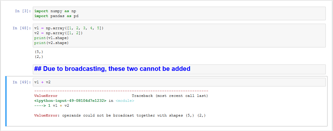
I could change the arrays to be multidimensional and reshape them to get the addition to happen. Doing so would be matrix addition though, and that’s not really the point. The takeaway is that these two one-dimensional arrays cannot be added together because their shapes don’t combine with broadcasting and element-wise processing.
R Vector Addition
In R programming, we see the concept of recycling implemented instead of a broadcasting failure. When given the following code:
y <- c(1, 2, 3, 4, 5)
q <- c(1, 2)
f <- y + q
print(f)
The result is:
[1] 2 4 4 6 6
The smaller array is recycled across the larger array’s axis until the last element (i.e. 5) is processed.
R Vector Multiplication
The constraints of broadcasting apply to NumPy array multiplication as they did in addition. Also, the use of recycling applies to R vector multiplication in the same way it it did with vector addition.
Using the same arrays as above:
m <- y * q
print(m)
The result is:
[1] 1 4 3 8 5
This again shows how the smaller array is distributed along the larger array until the last element in the larger array is processed.
That concludes this brief review of R Vector Operations.
Categories: R Programming
Leave a Reply