Understanding vectors in R programming is at the core of learning the language. In this post, I’ll touch on some of the basics of vector implementation in R and examples of useful functions such as c(), seq(), rep().

The official documentation for vectors in R can be found here https://cran.r-project.org/doc/manuals/r-release/R-intro.html#Simple-manipulations-numbers-and-vectors

All Variables in R are Vectors

Basically, all variables in R are vectors. This is validated by using the is.vector() function:

OneLenVec <- 99
OneLenVec
is.vector(OneLenVec)

This demonstrates that even a simple integer is represented as a vector:

The Combine Function

A simple way to create a vector with multiple members is by using the combine function.

> NumericVector <- c(78, 99, 1, -55, 22)
> print(NumericVector)
[1] 78 99 1 -55 22
> is.numeric(NumericVector)
[1] TRUE
> is.double(NumericVector)
[1] TRUE

Also seen above are some other new “is.XYZ” functions where the data type can be checked.

Vector Data Types are Homogeneous

A good example of how R handles mixed data types is vectors is seen below:

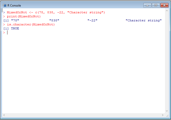
R converted all vector elements to character strings because one of the elements was a character string.

Creating Vectors with Seq and Rep

When I first saw the “X:Y” syntax in for loops, I immediately thought of Python. Previous notes on for loops are captured in this blog post. However, the “X:Y” syntax does not support a third value to specify step as is seen in Python. However, the seq() function also can be used to create vectors, and it does support the step option.

The basic use of the sequence function is as follows:

basic_sequence <- seq(1, 10)
print(basic_sequence)
[1] 1 2 3 4 5 6 7 8 9 10
seq_with_step <- seq(1, 10, 3)
print(seq_with_step)
[1] 1 4 7 10

The rep() function is used to replicate vectors. First, remember that all variables are vectors, so the rep() function can be used as shown below:

single_char <- “a”
ten_chars <- rep(single_char, 10)
print(ten_chars)
[1] “a” “a” “a” “a” “a” “a” “a” “a” “a” “a”

The function behaves, such that, it replicates the entire vector:

message <- c(“Replicate”, “me”)
print(rep(message, 3))
[1] “Replicate” “me” “Replicate” “me” “Replicate” “me”

Accessing Vector Elements

Vectors are indexed starting at 1 instead of 0. Using the previous vector, MixedOrNot, I can get the second element as follows:

MixedOrNot[2]
[1] “3943”

Another observation is the use of negative indexing. In Python, for example, imagine the following code:

python_array = [1, 2, 3, 4, 5, 6]
print(python_array[-3])

That will print the “negative 3rd indexed” item, which is 4.

In R, this actually removes the third item from the vector:

As expected, the “X:Y” syntax is supported (e.g. using r_vector) from the last screen shot:

print(r_vector[1:3])
[1] 1 2 3

There are some other creative ways to selectively pull elements from the vector. For example, to pull the first, third, and fifth element of a vector:

print(r_vector[c(1, 3, 5)])
[1] 1 3 5

The use of “X:Y”, combine c(), and related combinations provide a variety of ways to access elements of the vector.

This concludes the basic overview of vectors in R programming.

Categories: R Programming

Tags: R Programming, Software Development